One way ANOVA

Description

Like the Student’s t-Test, the one-way ANOVA (Analysis of Variance) test measures the differences between the means of groups, however, it looks for differences between more than two groups. This test assumes that the means are calculated from normally distributed data and that the groups are independent from each other. The p-value of the test will indicate whether there are any significant differences in the mean of individual groups as a whole but to identify whether these differences exist between individual/specific pairs, a post-hoc test such as Tukey’s Honesty test is required. Under the null hypothesis that all the means are not statistically different, if rejected we can conclude there is a statistical difference between at least 2 of the means but can not conclude which 2 (or more) average means are statistically different.

Benefits

Identifies differences in continuous variables across more than two categorical groups and prevents the need to conduct multiple t-tests (which also increases type 1/α error).

Drawbacks

ANOVA will only identify the presence of significant difference between one group/pair and requires post-hoc tests to identify the specific pairs that differ. Like t-test, it also requires a continuous variable that is normally distributed.

Worked Example

Download the example Excel file below.

The example here looks for differences in the temperatures measured by temperature probes A, B and C.

↬ Analyse

In the file there are several headed columns
- Whether the person has appendicitis or not
- Whether the temperature of the person is low, normal or high
Open rBiostatistics >> Comparative >> Mean >> One-way ANOVA >> Analyze
Browse and upload the Excel file
- Note that you must choose file type (.xlsx or .csv) as appropriate
- .csv files also need you to define your separator
Select the variable you would like to include in your analysis
Define the variables for both row and column
Various tabs are available to view the statistical output on the top
- Error bar and Box plot are also available
Results
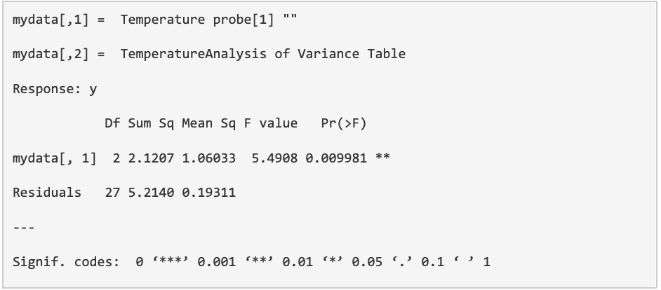
- Degree of freedom (df) = 2 and 27
- Sum of squares (Sum sq) = 2.121
- Mean square (Mean Sq)= 1.060
- F-statistic (F value) = 5.491
- p-value (Pr(>F)) = 0.010
Interpretation
- There is statistically significant differences between the probes when measuring temperature
Example of randomised dataset
- An extra column of randomised data has been included named “random temp”
- This means it is very unlikely to generate any statistically significant findings
- By running the same steps as above using the randomised numbers, the P value will be calculated as 0.2906, which is statistically insignificant